Kahan’s Summation Algorithm: Computing Better Sums

Suppose you have the following list of numbers in Python and you would like to compute the sum. You use the sum() function and expect it to return 0.3. Yet, when you run the code the console returns a value very slightly above 0.3:

numbers = [0.1, 0.1, 0.1]

sum(numbers)

0.30000000000000004

You can round this number of course, but it begs the question as to why the correct sum was not returned in the first place. Enter the IEEE 754 floating point standard.

Floating Point Storage

The double type is a 64 binary digit (bit) numerical storage standard that includes 1 sign bit (determines if number is positive or negative), a 53 bit significand (only 52 are stored for non-zero values), and an 11 bit exponent.

An 11 bit exponent means the smallest positive number that can be stored is 2-1022. Additionally, the largest rounding error possible in this standard is 2-52 called machine epsilon. Because this is a binary representation that means numbers that can be represented exactly in base 10 must be approximated when converting to binary.

Going back to our example above, 0.1 is a value that must be rounded for storage in this format. This is because 0.1 in binary is infinite:

0.000110011001100110011...

There are methods to store values exactly but this comes at the speed of computation. What if we want to keep the speed of 64 bit computation but reduce our error, specifically for large number series?

The Algorithm

Enter Kahan’s Summation Algorithm. Developed by William Kahan, this summation methodology allows for more accurate summation using the double storage format. Here is a simple Python implementation:

def kahan_sum(x):
   
  sum = 0.0
  c = 0.0
 
  for i in x:
    y = i - c
    t = sum + y
    c = t - sum - y
    sum = t
 
  return sum

Okay, so this looks pretty simple. But what do each of the pieces mean? The first two lines establish a function in Python while setting the starting sum and starting error to 0.0:

def kahan_sum(x):
   
  sum = 0.0
  c = 0.0

The next few lines are the for loop that iterates over each number in the list. First, any error is subtracted from the previous iteration.

y = i - c

Second, the new number is added to the running total minus any error.

t = sum + y

Third, error from this new addition is determined and the new total is assigned. This repeats until there are no more numbers.

c = t - sum - y
sum = t

A Practical Example

Okay, so the code is pretty simple but how does this work in practice? Suppose we have a list of two numbers:

[1.0, 1.0]

Step 1

The sum and error terms are set to 0.0 when the algorithm is started. The first step of each iteration is to take the current value and subtract any error from the previous iteration. Because the starting error is 0.0, we subtract 0.0 from the first value.

1.0 - 0.0 = 1.0

Step 2

Next we add the result of the previous operation to the total. Again, the initial total is 0.0 so we just add 0.0 to the value from Step 1 (1.0). Oh no! The computer had to make a rounding error. In this case, the computer was off by 0.1. We can handle this error in the next steps.

0.0 + 1.0 ~ 1.1

Step 3

In this step we determine the error from Step 2. We take the sum from Step 2 (1.1), subtract the total (0.0), and subtract the total from Step 1 (1.0). This leaves us with the approximate error.

1.1 - 0.0 - 1.0 ~ 0.1

Step 4

Finally, we record the current total for the next iteration!

1.1

And Repeat!

Now we repeat Steps 1, 2, 3, and 4 for each additional number. The difference this time is that we have non-zero values for the error and total terms. First, we subtract the error term from the last iteration to the new value:

1.0 - 0.1 = 0.9

Next, add the new value to the previous total:

1.1 + 0.9 = 2.0

Next, take the sum from the last step and subtract the previous iteration’s total and the value from the first step to estimate any error. In this case there is no error so we record a value of 0.0 for the error going into the next iteration:

2.0 - 1.1 - 0.9 = 0.0

Finally, return the sum. We can see that even though the computer made an error of 0.1, the algorithm corrected itself and returned the correct value:

2.0

Final Thoughts

Kahan’s method of summation strikes a balance between the speed of floating point arithmetic and accuracy. Hopefully this walkthrough makes the algorithm more approachable.

Association Rule Mining in R

Association rule mining is the process of determining conditional probabilities within events that contain items or characteristics. Events can range from tweets, to grocery store receipts, to credit card applications.

Items within these events should also not be unique to each event. For example, words are repeated across tweets, multiple customers will buy the same items at the grocery store, and credit card applicants will share specific characterisitcs.

For all of these applications our goal is to estimate the probability that an event will possess item B given that it has item A. This probability is also called the confidence.

In the example above we might say that we are 23% confident that a customer will purchase rice (item B) given they are purchasing chicken (item A). We can use historical transactions (events) to estimate confidence.

Now for a practical implementation using the tidyverse in R! I am using a groceries dataset from Georgia Tech. This dataset contains rows with items separated by commas.

receipt
citrus fruit, semi-finished bread
ready soups, margarine
One transaction per row with items comma separated.

Because each event contains different items I read it using readLines() and reshape into a longer format. The groceries column contains the item name while transaction contains the transaction ID.

link <- "https://cse6040.gatech.edu/datasets/groceries.csv"
groceries <- readLines(link)

# Create long form version of data
groceries_long <- 
  tibble::tibble(groceries) |>
  dplyr::mutate(
    transaction = dplyr::row_number()
  ) |>
  tidyr::separate_rows(
    groceries,
    sep = ","
  )
groceriestransaction
citrus fruit1
semi-finished bread1
tropical fruit2
Long form data with one item per row with a transaction ID.

With our data in the proper format we can develop two functions. The first function takes a vector of items and returns a vector of comma separated combinations as (A,B) and (B,A).

comb_vec <- function(items) {
  # Gets vector of all 2-level combinations
  
  p <- t(combn(items, 2))
  reg <- glue::glue("{p[, 1]},{p[, 2]}")
  rev <- glue::glue("{p[, 2]},{p[, 1]}")
  c(reg, rev)
}

For example, giving this function c("A", "B", "C") would return c("A,B" "A,C" "B,C" "B,A" "C,A" "C,B"). This is because we want to determine the probabilities of A given B and B given A.

Our final function performs the data mining. The first argument called data takes in the data frame of events and items. The last two arguments item_col and event_id tell the function which columns refer to the items and the event identifier respectively.

pair_assoc <- function(data, item_col, event_id, item_min = 1L) {
  # Derives association pairs for all elements in data
  
  # Count all items
  item_count <-
    data |>
    dplyr::count(
      A = {{ item_col }},
      name = "A Count"
    )
  
  # Get pairs as probabilities
  data |>
    dplyr::group_by({{ event_id }}) |>
    dplyr::filter(length({{ item_col }}) > 1) |>
    dplyr::reframe(comb = comb_vec({{ item_col }})) |>
    dplyr::ungroup() |>
    dplyr::count(
      comb,
      name = "A B Count"
    ) |>
    tidyr::separate(
      col = comb,
      into = c("A", "B"),
      sep = ","
    ) |>
    dplyr::left_join(
      y = item_count,
      by = "A"
    ) |>
    dplyr::mutate(
      Confidence = `A B Count` / `A Count`
    ) |>
    dplyr::arrange(desc(Confidence))
}

This function works in two stages. First, it determines the count of all individual items in the data set. In the example with groceries, this might be the counts of transactions with rice, beans, etc.

groceriesA Count
baking powder174
berries327
Counts of individual items serve as the denominator in the confidence computation.

The second stage uses the comb_vec() function to determine all valid item combinations within each group. This stage only returns valid combinations where the confidence is > 0%.

Finally, the function left joins the item counts to the combination counts and computes the confidence values. I called the function and return the result. I am also filtering to only combinations with a confidence of 50% or more with items purchased more than 10 times.

groceries_long |>
  pair_assoc(
    item_col = groceries, 
    event_id = transaction
  ) |>
  dplyr::filter(
    `A Count` >= 10,
    Confidence >= 0.5
  )

Here we can see the head of the results table ordered by confidence from highest to lowest. We observe that the confidence of honey and whole milk is 73%! In other words, 73% of the transactions that contain honey also contain whole milk.

ABA B CountA CountConfidence
honeywhole milk11140.733
frozen fruitsother vegetables8120.667
cerealswhole milk36560.643
ricewhole milk46750.613
Head of results table.

Association rule mining is a fairly simple and easy to interpret technique to help draw relationships between items and events in a data set.

The Logistic Map: Visualizing Chaos in R

In the 1970s, professor Robert May became interested in the relationship between complexity and stability in animal populations. He noted that even simple equations used to model populations over time can lead to chaotic outcomes. The most famous of these equations is as follows:

xn+1 = rxn(1 – xn)

xn is a number between 0 and 1 that refers to the ratio of the existing population to the maximum possible population. Additionally, r refers to a value between 0 and 4 which indicates the growth rate over time. xn is multiplied by the r value to simulate growth where (1 – xn) represents death in the population.

Lets assume a population of animals is at 50% of the maximum population for a given area. We would allow xn to be .5. Lets also assume a growth rate of 75% allowing r to be .75. After the value xn+1 is computed, we use that new value as the xn in the next iteration and continue to use an r value of .75. We can visualize how xn+1 changes over time.

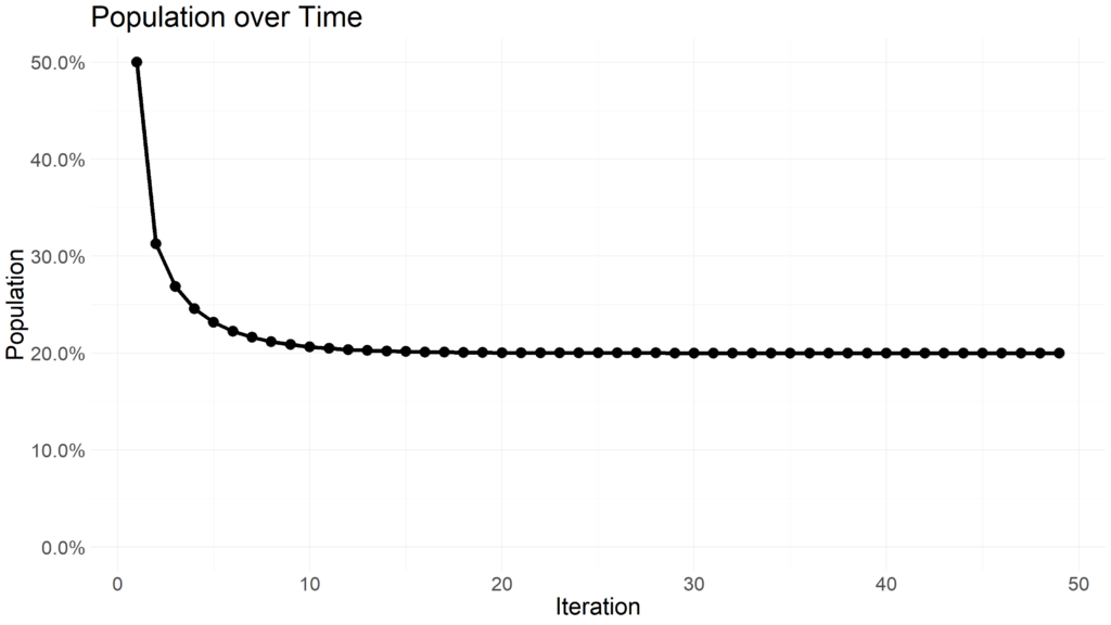
Visualizing the population with an r value of 50% and a starting population of 50%.

Within 20 iterations, the population dies off. Lets rerun the simulation with an r value greater than 1.

Visualizing the population with an r value of 1.25 and a starting population of 50%.

Notice how the population stabilizes at 20% of the area capacity. When the r value is higher than 3, the population with begin oscillating between multiple values.

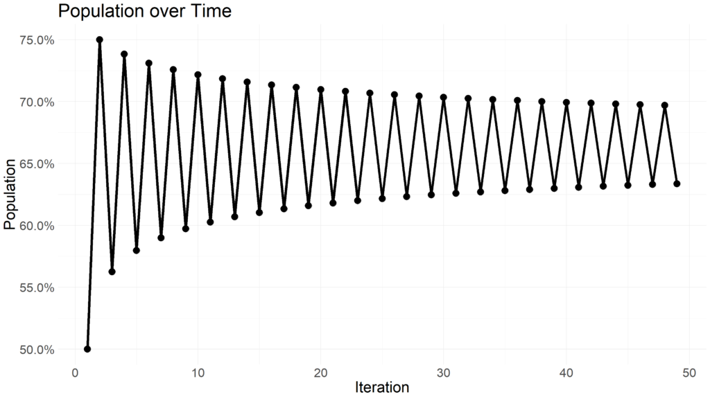
Visualizing the population with an r value of 3 and a starting population of 50%.

Expanding beyond an r value of 3.54409 yields rapid changes in oscillation and reveals chaotic behavior.

Visualizing the population with an r value of 3.7 and a starting population of 50%.

Extremely minor changes in the r value yield vastly different distributions of population oscillations. Rather than experiment with different r values, we can visualize the distribution of xn+1 values for a range of r values using the R programming language.

Lets start by building a function in R that returns the first 1000 iterations of xn+1 for a given r value.

logistic_sim <- function(lamda, starting_x = 0.5) {
  # Simulate logistic function
  
  vals <- c(starting_x)
  iter <- seq(1, 1000, 1)
  
  for (i in iter) { 
    vals[(i + 1)] <- vals[i] * lamda * (1 - vals[i])
  }
  
  vals <- vals[-length(vals)]
  tibble::tibble(vals, lamda, iter)
}

This function returns a dataframe with three columns: the iteration number, the r used for each iteration, and the xn+1 value computed for that iteration.

Now we need to iterate this function over a range of r values. Using purrr::map_dfr we can row bind each iteration of r together into a final dataframe.

build_data <- function(min, max) {
  # Build data for logistic map
  
  step <- (max - min) / 400
  
  purrr::map(
    seq(min, max, step),
    logistic_sim
  ) |>
    purrr::list_rbind()
}

Min refers to the lower limit of r while the max refers to the upper limit. The function will return a dataframe of approximately 400,000 values referring to each of the 1000 iterations for the 400 r values between the lower and upper bound. The function returns all 400,000 values in less than a quarter of a second.

With the dataframe of values assembled, we can visualize the distribution of values using ggplot.

build_data(1, 4) |>
  dplyr::filter(iter > 50) |>
  dplyr::slice_sample(prop = 0.1) |>
  ggplot2::ggplot(aes(
    x = lamda,
    y = vals,
    color = lamda
  )) +
  ggplot2::geom_point(size = 0.5) +
  ggplot2::labs(
    x = "Growth Rate",
    y = "Population Capacity",
    title = "Testing Logistic Growth in Chaos"
  ) +
  ggplot2::scale_x_continuous(
    labels = scales::percent
  ) +
  ggplot2::scale_y_continuous(
    labels = scales::percent
  ) +
  ggplot2::theme_minimal() +
  ggplot2::theme(
    legend.position = "none",
    text = element_text(size = 25)
  )
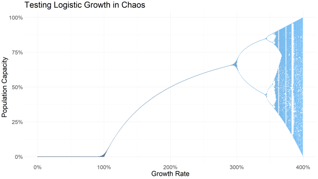
Visualizing the distribution of 400 r values between 0 to 4 for 1000 iterations.

Notice how r values of less than 1 indicate the population dies out. Between 1 and just under three, the population remains relatively stable. At around 3, the populations being oscillating between two points. Beyond an r of 3.54409, chaos ensues. It becomes extremely difficult to predict the value of xn+1 for a given iteration with an r value above 3.54409. So difficult, in fact, that this simple deterministic equation was used as an early random number generator.

So what are the practical applications for this? Representations of chaos (or systems that yield unpredictable results and are sensitive to starting conditions) can be seen across many industries and fields of study. In finance, for example, intra-day security prices have been described as a random walk – extremely difficult to predict. While long term outlooks may show seasonality, chaos theory can help model the extremely chaotic and unpredictable nature of stock prices.

Implementing Fuzzy Matching in Python

Text is all around us; essays, articles, legal documents, text messages, and news headlines are consistently present in our daily lives. This abundance of text provides ample opportunities to analyze unstructured data.


Imagine you are playing a game where someone hands you a index card with the misspelled name of a popular musician. In addition, you have a book containing correctly spelled names of popular musicians. The goal is for you to return the correct spelling of the misspelled name.

In this example, suppose someone hands you a card with “Billie Jole” written on it. You quickly open the book of musicians, find names beginning with the letter B, and find the name “Billy Joel.”

As a human, this was easy for you to complete, but what if you wanted to automate this task? This can be done using Fuzzy Logic, or more specifically, the Levenshtein distance.


The Levenshtein distance considers two pieces of text and determines the minimum number of changes required to convert one string into another. You can utilize this logic to find the closest match to any given piece of text.

I am going to focus on implementing the mechanics of finding a Levenshtein distance in Python rather than the math that makes it possible. There are many resources on YouTube which explain how the Levenshtein distance is calculated.


First, import numpy and define a function. I called the function lv as shorthand for Levenshtein distance. Our function requires two input strings which are used to create a 2D matrix that is one greater than the length of each string.

def ld(s1, s2):    
    rows = len(s1)+1
    cols = len(s2)+1
    dist = np.zeros([rows,cols])

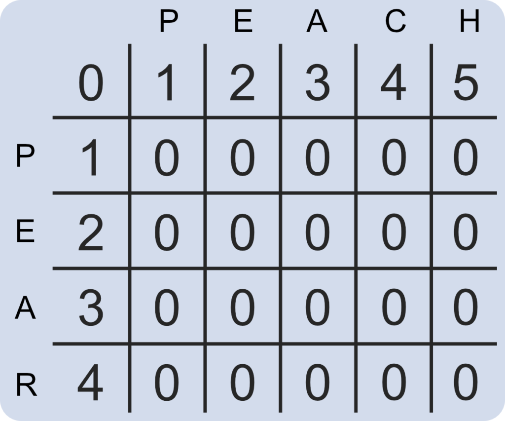
If you were to use the strings “pear” and “peach” in this instance, the function should create a 5 by 6 matrix filled with zeros.

A matrix of zeros.

Next, the first row and column need to count up from zero. Using for loops, we can iterate over the selected values. Our Python function now creates the following matrix.

def ld(s1, s2):
    rows = len(s1)+1
    cols = len(s2)+1
    dist = np.zeros([rows,cols])
    
    for i in range(1, rows):
        dist[i][0] = i
    for i in range(1, cols):
        dist[0][i] = i
A matrix set up for finding the Levenshtein distance.

Finally, we need to iterate over every column and row combination. By doing this, we can find the minimum value of the cells directly above, to the left, and above to the left of each cell. After the minimum is found, our Python script adds one to this value to the location in question.

def ld(s1, s2):
    rows = len(s1)+1
    cols = len(s2)+1
    dist = np.zeros([rows,cols])
    
    for i in range(1, rows):
        dist[i][0] = i
    for i in range(1, cols):
        dist[0][i] = i
        
    for col in range(1, cols):
        for row in range(1, rows):
            if s1[row-1] == s2[col-1]:
                cost = 0
            else:
                cost = 1
            dist[row][col] = min(dist[row-1][col] + 1,
                                 dist[row][col-1] + 1,      
                                 dist[row-1][col-1] + cost)
            return dist[-1][-1]

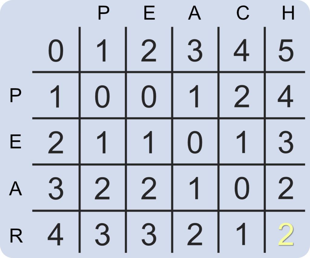
Our matrix should now look like the following with the far bottom right cell representing the number of changes required to convert one string into another. In this instance, it requires 2 changes to convert “peach” into “pear”; deleting the letter “c” in “peach” and replacing the letter “h” with the letter “r”.

A completed Levenshtein distance matrix. The bottom right number (in gold) represents the number of changes required.

What is so great about this function is that it is adaptable and will accept a string of any length to compute the number of changes required. While the mechanics behind this function are relatively simple, its use cases are vast.

Hi! I’m Chris Walker.

I am a Senior Data Scientist at Fannie Mae. I have an MS in Analytics from Georgia Tech. Additionally, I graduated from Texas A&M University with a BS in Urban and Regional Planning with a minor in Economics. I am excited about housing, risk modeling, and data science.

Feel free to contact me on LinkedIn or via email at walkerjameschris@gmail.com