Advent of Code 2023: Day Three

Advent of Code is an annual series of holiday themed programming challenges which can be completed in any language. There is one problem for each day in December before Christmas!

Day three asks us to consider an engine schematic which needs to be parsed. If a symbol has a number adjacent to it (could be horizontal, vertical, or diagonal) we need to keep it. We sum up all numbers at the end to identify the missing part number. You can see the original problem here.

In the text below, we can see symbols (any value that is not a period or a number). The first star on the second row means that the number 467 is considered but the number 114 is not considered since no part of the number is directly adjacent.

467..114..
...*......
..35..633.
......#...
617*......
.....+.58.
..592.....
......755.
...$.*....
.664.598..

I decided to use R and the tidyverse to solve this problem. The real schematic is much larger than the example shown above. First, I load the text and parse the lines into a useful tibble format.

#### Setup ####

library(tidyr)
library(dplyr)
library(readr)
library(tibble)

lines <- readr::read_lines("~/Documents/data.txt")

digits <- seq(0, 9)
non_symbols <- c(".", digits)

#### Parse Schematic ####

parsed_lines <-
  lines |>
  stringr::str_split("") |>
  purrr::imap(function(value, row) {
    
    tibble::tibble(
      row,
      col = seq_along(value),
      value
    )
    
  }) |>
  dplyr::bind_rows()
  
# A tibble: 19,600 × 3
#   row   col value
#   <int> <int> <chr>
# 1     1     1  .    
# 2     1     2  .    
# 3     1     3  .    
# 4     1     4  .    
# 5     1     5  5    
# 6     1     6  7    
# 7     1     7  3    
# 8     1     8  .    
# 9     1     9  6    
# 10    1    10  1    
# ℹ 19,590 more rows

Next, I parse this data frame into two pieces, symbols and numbers. I want to determine the row-column positions of each number as an instance instead of individual characters. I use the lag function to determine the extent of a number and store these for later use.

number_df <-
  parsed_lines |>
  dplyr::mutate(
    is_num = value %in% digits,
    num_instance = cumsum(is_num != lag(is_num, 1, FALSE))
  ) |>
  dplyr::filter(
    value %in% digits
  ) |>
  dplyr::group_by(num_instance) |>
  dplyr::mutate(
    number = glue::glue_collapse(value)
  ) |>
  dplyr::ungroup() |>
  dplyr::select(
    row,
    col,
    number,
    num_instance
  )

I also parse the symbols. I first identify any character which is not a number or a period. Next, I expand to a series of nudges or adjustments to the row-column pair in all directions where a potential number could be matched.

nudges <-
  tidyr::expand_grid(
    col_nudge = seq(-1, 1),
    row_nudge = seq(-1, 1)
  ) |>
  dplyr::filter(
    !(col_nudge == 0 & row_nudge == 0)
  )

symbol_df <-
  parsed_lines |>
  dplyr::filter(
    !value %in% non_symbols
  ) |>
  dplyr::mutate(
    sym_instance = row_number()
  ) |>
  tidyr::expand_grid(nudges) |>
  dplyr::mutate(
    row = row + row_nudge,
    col = col + col_nudge
  )

Finally, I join these together an ensure that only one instance of a number is present for each symbol (so numbers which are both horizontally and vertically above a symbol are not double counted, for example). This allows me to take the simple sun and find the answer which is 560670! On my machine this implementation takes around 150ms which is fairly quick!

symbol_df |>
  dplyr::inner_join(
    y = number_df,
    by = c("row", "col")
  ) |>
  dplyr::distinct(
    number,
    sym_instance,
    num_instance
  ) |>
  dplyr::pull(number) |>
  as.numeric() |>
  sum()

High Performance Scientific Computing with Rcpp

In data science we often face a tradeoff between run time and development time when it comes to our choice of language. Languages like R and Python are common because they are easy to write, even if the language runtime is slow.

In some cases, writing R is only slightly more verbose than the comparable statement in English. For example, suppose we wanted to take some data, filter to where x is greater than 2, and find the mean of column y. We could write this in R as follows:

library(tidyverse)

data |>
  dplyr::filter(x > 2) |>
  dplyr::reframe(
    new_col = mean(y)
  )

This brutal simplicity comes at at the expense of speed in some cases. Often times we prefer ease of use to speed, but what if speed is critical! We might need to use a language like C++ or Rust but this comes with added complexity – how do we use C++ in components of our workflow and R in others? How is data transfer handled between these environments? How do I compile code effectively?

Enter Rcpp, a fantastic tool which strips away almost all of the barriers to entry with C++ when coming from R. This R package allows users to write C++ functions which accept R objects to be processed in C++ and returned in R. It handles all of the complexities of data transfer and object serialization.


Lets take an example in R. Suppose we wanted to compute the mean across several columns. In other words, what is the mean of the ith element of a collection of column vectors? The tidyverse includes a function called dplyr::rowwise() specifically designed for this purpose. While exceptionally general, it is painfully slow. Lets write a C++ function to help us out.

The snippet below is the contents of a file called functions.cpp, a C++ file which contains a function called row_means_cpp(). This function accepts a 2D matrix and returns a column vector.

It iterates over each row finding the mean across all columns in this dataset. We begin by determining the shape of the matrix, looping over the rows and columns while computing the means along the way, and returning the vector.

#include <Rcpp.h>
using namespace Rcpp;

// [[Rcpp::export]]
NumericVector row_means_cpp(NumericMatrix X) {

  int row = X.nrow();
  int col = X.ncol();
  NumericVector result(row);
  
  for (int i = 0; i < row; i++) {
  
    double mean = 0;
  
    for (int j = 0; j < col; j++) {
      mean += X(i, j);
    }
    
    result[i] = mean / col;
  }

  return result;
}

Now lets see how this compares to the dplyr function in R! We can use the bench package to profile R expressions. I have also designed a wrapper R function around our C++ function to make workflows with data frames a little easier called row_means().

library(Rcpp)
library(bench)
library(ggplot2)

Rcpp::sourceCpp("functions.cpp")

row_means <- function(...) {

  list(...) |>
    as.data.frame() |>
    as.matrix() |>
    row_means_cpp()
    
}

bench::mark(
  Rowwise = {
  
    diamonds |>
      dplyr::rowwise() |>
      dplyr::mutate(
        means = mean(c(carat, depth, table, price, x, y, z))
      )
  
  },
  Cpp = {
  
    diamonds |>
      dplyr::mutate(
        means = row_means(carat, depth, table, price, x, y, z)
      )
  
  },
  check = FALSE
) |>
  dplyr::select(
    expression,
    median,
    mem_alloc
  ) |>
  print()

# A tibble: 2 × 3
  expression   median mem_alloc
  <bch:expr> <bch:tm> <bch:byt>
1 Rowwise    651.25ms   28.08MB
2 Cpp          2.37ms    3.44MB

We compute the row-wise mean of seven columns. Specifically, the means of carat, depth, table, price, x, y, and z. We can see in the tibble output above that the dplyr version is approximately 300 times slower and 8 times less memory efficient than our C++ function!

While the C++ function is markedly less general, for specific workflows it might represent a meaningful improvement in speed and performance. This makes Rcpp an excellent candidate for tinkering with machine learning models from scratch in R! You can implement machine learning models with fast procedural C++ code with the ease of scripting in R – a fantastic duo!

Create Validated Data in R with dataclass

dataclass is an R package I created to easily define templates for lists and data frames that validate each element. This package is useful for validating data within R processes which pull from dynamic data sources such as databases and web APIs to provide an extra layer of validation around input and output data.

To use dataclass you specify the expected type, length, range, allowable values, and more for each element in your data. Decide whether violations of these expectations should throw an error or a warning.

For example, suppose you wanted to create a data frame in R which contains three columns: date, low_flag, and metric. These columns represent the output of some analytic process in R. Traditionally, you would simply write these columns as a data frame. How can we be sure that the data is correct? Simply describe your data in a declarative fashion:

library(dataclass)

my_dataclass <-
  dataclass::dataclass(
    # Date, logical, and numeric column
    date = dataclass::dte_vec(),
    low_flag = dataclass::lgl_vec(),
    metric = dataclass::num_vec()
  ) |>
  dataclass::data_validator()

Now we have a template for our data called my_dataclass. Because we want to validate a data frame (as opposed to a list) we called data_validator() to let dataclass know we are validating a data frame. How do we use it? Simply pass your data to validate as a function. If we pass in valid inputs, dataclass returns the input data. However, invalid inputs throw an error.

tibble::tibble(
  date = Sys.Date(),
  low_flag = TRUE,
  metric = 1
) |>
  my_dataclass()
  
#> # A tibble: 1 × 3
#>   date       low_flag metric
#>   <date>     <lgl>     <dbl>
#> 1 2023-03-21 TRUE          1

tibble::tibble(
  date = Sys.Date(),
  low_flag = TRUE,
  metric = "A string!"
) |>
  my_dataclass()
  
#> Error:
#>   ! The following elements have error-level violations:
#>   ✖ metric: is not numeric
#> Run `rlang::last_error()` to see where the error occurred.

We can also use dataclass to validate lists. Suppose we want to validate that a list contains date, my_data, and note where these elements correspond to the run date, a data frame, and a string respectively:

new_dataclass <-
  dataclass::dataclass(
    date = dataclass::dte_vec(1),
    my_data = dataclass::df_like(),
    note = dataclass::chr_vec(1)
  )

Now we can validate a list!

new_dataclass(
  date = Sys.Date(),
  my_data = head(mtcars, 2),
  note = "A note!"
)

#> $date
#> [1] "2023-03-21"
#> 
#> $my_data
#> mpg cyl disp  hp drat    wt  qsec vs am gear carb
#> Mazda RX4      21   6  160 110  3.9 2.620 16.46  0  1    4    4
#> Mazda RX4 Wag  21   6  160 110  3.9 2.875 17.02  0  1    4    4
#> 
#> $note
#> [1] "A note!"

new_dataclass(
  date = Sys.Date(),
  my_data = mtcars,
  # note is not a single string!
  note = c(1, 2, 3)
)

#> Error:
#>   ! The following elements have error-level violations:
#>   ✖ note: is not a character
#> Run `rlang::last_error()` to see where the error occurred.

And that’s it! It’s pretty easy and minimal to get started. The learning curve is very minimal while the benefits of data validation cannot be overstated in a data science workflow!

You can install dataclass from CRAN by running the command below in your R console. Finally, if you want to contribute or submit bugs you can visit the GitHub repository here.

install.packages("dataclass")

Association Rule Mining in R

Association rule mining is the process of determining conditional probabilities within events that contain items or characteristics. Events can range from tweets, to grocery store receipts, to credit card applications.

Items within these events should also not be unique to each event. For example, words are repeated across tweets, multiple customers will buy the same items at the grocery store, and credit card applicants will share specific characterisitcs.

For all of these applications our goal is to estimate the probability that an event will possess item B given that it has item A. This probability is also called the confidence.

In the example above we might say that we are 23% confident that a customer will purchase rice (item B) given they are purchasing chicken (item A). We can use historical transactions (events) to estimate confidence.

Now for a practical implementation using the tidyverse in R! I am using a groceries dataset from Georgia Tech. This dataset contains rows with items separated by commas.

receipt
citrus fruit, semi-finished bread
ready soups, margarine
One transaction per row with items comma separated.

Because each event contains different items I read it using readLines() and reshape into a longer format. The groceries column contains the item name while transaction contains the transaction ID.

link <- "https://cse6040.gatech.edu/datasets/groceries.csv"
groceries <- readLines(link)

# Create long form version of data
groceries_long <- 
  tibble::tibble(groceries) |>
  dplyr::mutate(
    transaction = dplyr::row_number()
  ) |>
  tidyr::separate_rows(
    groceries,
    sep = ","
  )
groceriestransaction
citrus fruit1
semi-finished bread1
tropical fruit2
Long form data with one item per row with a transaction ID.

With our data in the proper format we can develop two functions. The first function takes a vector of items and returns a vector of comma separated combinations as (A,B) and (B,A).

comb_vec <- function(items) {
  # Gets vector of all 2-level combinations
  
  p <- t(combn(items, 2))
  reg <- glue::glue("{p[, 1]},{p[, 2]}")
  rev <- glue::glue("{p[, 2]},{p[, 1]}")
  c(reg, rev)
}

For example, giving this function c("A", "B", "C") would return c("A,B" "A,C" "B,C" "B,A" "C,A" "C,B"). This is because we want to determine the probabilities of A given B and B given A.

Our final function performs the data mining. The first argument called data takes in the data frame of events and items. The last two arguments item_col and event_id tell the function which columns refer to the items and the event identifier respectively.

pair_assoc <- function(data, item_col, event_id, item_min = 1L) {
  # Derives association pairs for all elements in data
  
  # Count all items
  item_count <-
    data |>
    dplyr::count(
      A = {{ item_col }},
      name = "A Count"
    )
  
  # Get pairs as probabilities
  data |>
    dplyr::group_by({{ event_id }}) |>
    dplyr::filter(length({{ item_col }}) > 1) |>
    dplyr::reframe(comb = comb_vec({{ item_col }})) |>
    dplyr::ungroup() |>
    dplyr::count(
      comb,
      name = "A B Count"
    ) |>
    tidyr::separate(
      col = comb,
      into = c("A", "B"),
      sep = ","
    ) |>
    dplyr::left_join(
      y = item_count,
      by = "A"
    ) |>
    dplyr::mutate(
      Confidence = `A B Count` / `A Count`
    ) |>
    dplyr::arrange(desc(Confidence))
}

This function works in two stages. First, it determines the count of all individual items in the data set. In the example with groceries, this might be the counts of transactions with rice, beans, etc.

groceriesA Count
baking powder174
berries327
Counts of individual items serve as the denominator in the confidence computation.

The second stage uses the comb_vec() function to determine all valid item combinations within each group. This stage only returns valid combinations where the confidence is > 0%.

Finally, the function left joins the item counts to the combination counts and computes the confidence values. I called the function and return the result. I am also filtering to only combinations with a confidence of 50% or more with items purchased more than 10 times.

groceries_long |>
  pair_assoc(
    item_col = groceries, 
    event_id = transaction
  ) |>
  dplyr::filter(
    `A Count` >= 10,
    Confidence >= 0.5
  )

Here we can see the head of the results table ordered by confidence from highest to lowest. We observe that the confidence of honey and whole milk is 73%! In other words, 73% of the transactions that contain honey also contain whole milk.

ABA B CountA CountConfidence
honeywhole milk11140.733
frozen fruitsother vegetables8120.667
cerealswhole milk36560.643
ricewhole milk46750.613
Head of results table.

Association rule mining is a fairly simple and easy to interpret technique to help draw relationships between items and events in a data set.

The Logistic Map: Visualizing Chaos in R

In the 1970s, professor Robert May became interested in the relationship between complexity and stability in animal populations. He noted that even simple equations used to model populations over time can lead to chaotic outcomes. The most famous of these equations is as follows:

xn+1 = rxn(1 – xn)

xn is a number between 0 and 1 that refers to the ratio of the existing population to the maximum possible population. Additionally, r refers to a value between 0 and 4 which indicates the growth rate over time. xn is multiplied by the r value to simulate growth where (1 – xn) represents death in the population.

Lets assume a population of animals is at 50% of the maximum population for a given area. We would allow xn to be .5. Lets also assume a growth rate of 75% allowing r to be .75. After the value xn+1 is computed, we use that new value as the xn in the next iteration and continue to use an r value of .75. We can visualize how xn+1 changes over time.

Visualizing the population with an r value of 50% and a starting population of 50%.

Within 20 iterations, the population dies off. Lets rerun the simulation with an r value greater than 1.

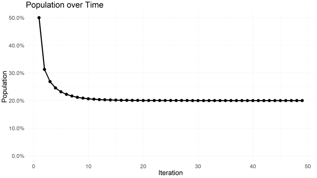
Visualizing the population with an r value of 1.25 and a starting population of 50%.

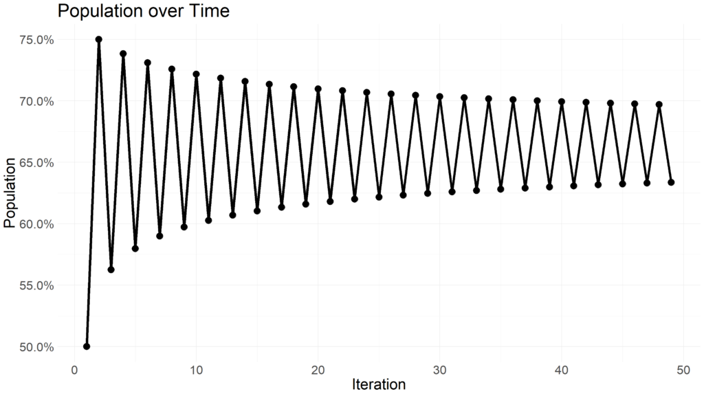
Notice how the population stabilizes at 20% of the area capacity. When the r value is higher than 3, the population with begin oscillating between multiple values.

Visualizing the population with an r value of 3 and a starting population of 50%.

Expanding beyond an r value of 3.54409 yields rapid changes in oscillation and reveals chaotic behavior.

Visualizing the population with an r value of 3.7 and a starting population of 50%.

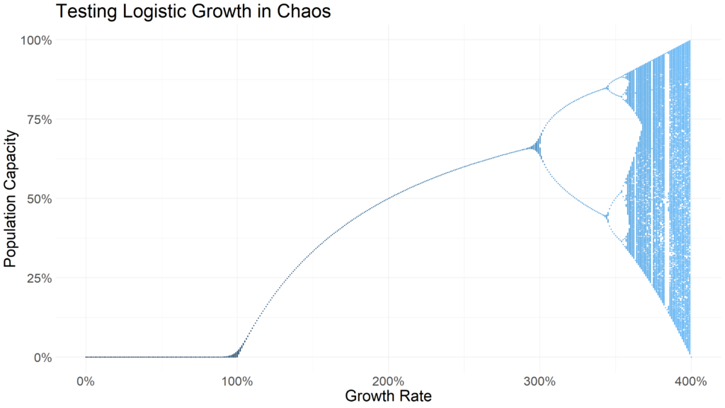
Extremely minor changes in the r value yield vastly different distributions of population oscillations. Rather than experiment with different r values, we can visualize the distribution of xn+1 values for a range of r values using the R programming language.

Lets start by building a function in R that returns the first 1000 iterations of xn+1 for a given r value.

logistic_sim <- function(lamda, starting_x = 0.5) {
  # Simulate logistic function
  
  vals <- c(starting_x)
  iter <- seq(1, 1000, 1)
  
  for (i in iter) { 
    vals[(i + 1)] <- vals[i] * lamda * (1 - vals[i])
  }
  
  vals <- vals[-length(vals)]
  tibble::tibble(vals, lamda, iter)
}

This function returns a dataframe with three columns: the iteration number, the r used for each iteration, and the xn+1 value computed for that iteration.

Now we need to iterate this function over a range of r values. Using purrr::map_dfr we can row bind each iteration of r together into a final dataframe.

build_data <- function(min, max) {
  # Build data for logistic map
  
  step <- (max - min) / 400
  
  purrr::map(
    seq(min, max, step),
    logistic_sim
  ) |>
    purrr::list_rbind()
}

Min refers to the lower limit of r while the max refers to the upper limit. The function will return a dataframe of approximately 400,000 values referring to each of the 1000 iterations for the 400 r values between the lower and upper bound. The function returns all 400,000 values in less than a quarter of a second.

With the dataframe of values assembled, we can visualize the distribution of values using ggplot.

build_data(1, 4) |>
  dplyr::filter(iter > 50) |>
  dplyr::slice_sample(prop = 0.1) |>
  ggplot2::ggplot(aes(
    x = lamda,
    y = vals,
    color = lamda
  )) +
  ggplot2::geom_point(size = 0.5) +
  ggplot2::labs(
    x = "Growth Rate",
    y = "Population Capacity",
    title = "Testing Logistic Growth in Chaos"
  ) +
  ggplot2::scale_x_continuous(
    labels = scales::percent
  ) +
  ggplot2::scale_y_continuous(
    labels = scales::percent
  ) +
  ggplot2::theme_minimal() +
  ggplot2::theme(
    legend.position = "none",
    text = element_text(size = 25)
  )
Visualizing the distribution of 400 r values between 0 to 4 for 1000 iterations.

Notice how r values of less than 1 indicate the population dies out. Between 1 and just under three, the population remains relatively stable. At around 3, the populations being oscillating between two points. Beyond an r of 3.54409, chaos ensues. It becomes extremely difficult to predict the value of xn+1 for a given iteration with an r value above 3.54409. So difficult, in fact, that this simple deterministic equation was used as an early random number generator.

So what are the practical applications for this? Representations of chaos (or systems that yield unpredictable results and are sensitive to starting conditions) can be seen across many industries and fields of study. In finance, for example, intra-day security prices have been described as a random walk – extremely difficult to predict. While long term outlooks may show seasonality, chaos theory can help model the extremely chaotic and unpredictable nature of stock prices.