Random Number Generation

Random number generators are at the core of many applied computer science applications. For example, stochastic simulation models, statistical sampling, and learning techniques all rely on random numbers generated by computers. However, computers are famously not random.

Computers allow us to reproduce complex calculations and workflows repeatedly and achieve the same result. So how can a machine which is designed to follow careful instruction generate randomness?

In fact, the random numbers generated by computers are not random at all. They leverage some starting point (a seed) and generate a series of numbers which follow that appear to have no relation to each other. However, if the same seed is used again the computer can generate the same series of numbers!

This is powerful because it means we can both simulate randomness, but also simulate that same randomness again in the future. But how do we generate random numbers and what form do those numbers take?


Sometimes we need to generate random whole numbers. Other times we need to generate percentages as a value between 0 and 1. And sometimes we need to generate random numbers which follow some distribution (say an exponential).

It turns out that as long as we can generate random numbers between 0 and 1, we can transform them to any reasonable distribution via the inverse transform theorem (this is something I might discuss in a future post). However, for now lets focus on random numbers between 0 and 1.

The most common random number generator is called the linear congruential generator or LCG. This class of generators has the following form (where U is one random value between 0 and 1):

X_{i}=aX_{i-1}+c \mod m

U_i=\frac{X_i}{m}

The values of a, c, and, m are all carefully chosen. There are two critical tests a random number generator must pass to be useful; independence and uniformity. We test that using runs and chi-squared tests, respectively.

An independence test verifies that the next value cannot be predicted by the current value. We say that a random number generator produces independent numbers if the following statement is true. Here A is the number of runs within a random number set.

\text{Independence:} \frac{A-\frac{2n-1}{3}}{\sqrt{\frac{16n-29}{90}}} < z_{0.975}

A run is simply continuous increases or decreases in values. For example: 1, 2, 3, 4, 3 has two runs because it counts up to four (the first run) and back down to three (the second run).

Next we test for uniformity. This sorts all values into buckets and counts them. If we had 1000 random numbers between 0 and 1 and we split them into quartiles we would expect (shown as E here) 250 values in each bucket. The O here is the number of observed values in those buckets.

\text{Uniformity:}\sum\frac{(O-E)^2}{E}<\chi_{0.95,k-1}^2

We can write a little bit of R to help us verify the performance of one very famous random number generator called the desert island generator. This generator chooses the values of 16807, 0, and 2147483647 for a, c, and m, respectively.


random <- function(n, seed = 123) {
  
  values <- numeric(n)
  m <- 2147483647
  
  for (i in seq(n)) {
    seed <- (16807 * seed) %% m
    values[i] <- seed / m
  }
  
  values
}

is_independent <- function(x, alpha = 0.95) {
  
  a <- head(x, -1)
  b <- tail(x, -1)
  
  change <- a > b
  run_change <- change != dplyr::lag(change, 1, 0)
  runs <- max(cumsum(x) + 1)
  
  n <- length(x)
  e <- (2 * n - 1) / 3
  v <- (16 * n - 29) / 90
  
  stat <- round(abs((runs - e) / (v ^ 0.5)), 2)
  crit <- round(qnorm(1 - (alpha / 2)), 2)
  
  msg <- dplyr::if_else(
    stat < crit,
    "Not Independent (Reject",
    "Independent (Accept"
  )
  
  glue::glue("{msg} H0): Stat = {stat}, Critical = {crit}")
}

is_uniform <- function(x, n = 100, alpha = 0.95) {
  
  e <- ceiling(length(x) / n)
  
  stat <- round(sum(((table(ceiling(x * n)) - e) ^ 2) / e), 2)
  crit <- round(qchisq(1 - alpha, n - 1), 2)
  
  msg <- dplyr::if_else(
    stat < crit,
    "Not Independent (Reject",
    "Independent (Accept"
  )
  
  glue::glue("{msg} H0): Stat = {stat}, Critical = {crit}")
}

x <- random(1e6)

is_independent(x)
# > Independent (Accept H0): Stat = 394.49, Critical = 0.06

is_uniform(x)
# > Independent (Accept H0): Stat = 128.36, Critical = 77.05

This implementation tests and verifies that our generator is random for 1M random values!

High Performance Scientific Computing with Rcpp

In data science we often face a tradeoff between run time and development time when it comes to our choice of language. Languages like R and Python are common because they are easy to write, even if the language runtime is slow.

In some cases, writing R is only slightly more verbose than the comparable statement in English. For example, suppose we wanted to take some data, filter to where x is greater than 2, and find the mean of column y. We could write this in R as follows:

library(tidyverse)

data |>
  dplyr::filter(x > 2) |>
  dplyr::reframe(
    new_col = mean(y)
  )

This brutal simplicity comes at at the expense of speed in some cases. Often times we prefer ease of use to speed, but what if speed is critical! We might need to use a language like C++ or Rust but this comes with added complexity – how do we use C++ in components of our workflow and R in others? How is data transfer handled between these environments? How do I compile code effectively?

Enter Rcpp, a fantastic tool which strips away almost all of the barriers to entry with C++ when coming from R. This R package allows users to write C++ functions which accept R objects to be processed in C++ and returned in R. It handles all of the complexities of data transfer and object serialization.


Lets take an example in R. Suppose we wanted to compute the mean across several columns. In other words, what is the mean of the ith element of a collection of column vectors? The tidyverse includes a function called dplyr::rowwise() specifically designed for this purpose. While exceptionally general, it is painfully slow. Lets write a C++ function to help us out.

The snippet below is the contents of a file called functions.cpp, a C++ file which contains a function called row_means_cpp(). This function accepts a 2D matrix and returns a column vector.

It iterates over each row finding the mean across all columns in this dataset. We begin by determining the shape of the matrix, looping over the rows and columns while computing the means along the way, and returning the vector.

#include <Rcpp.h>
using namespace Rcpp;

// [[Rcpp::export]]
NumericVector row_means_cpp(NumericMatrix X) {

  int row = X.nrow();
  int col = X.ncol();
  NumericVector result(row);
  
  for (int i = 0; i < row; i++) {
  
    double mean = 0;
  
    for (int j = 0; j < col; j++) {
      mean += X(i, j);
    }
    
    result[i] = mean / col;
  }

  return result;
}

Now lets see how this compares to the dplyr function in R! We can use the bench package to profile R expressions. I have also designed a wrapper R function around our C++ function to make workflows with data frames a little easier called row_means().

library(Rcpp)
library(bench)
library(ggplot2)

Rcpp::sourceCpp("functions.cpp")

row_means <- function(...) {

  list(...) |>
    as.data.frame() |>
    as.matrix() |>
    row_means_cpp()
    
}

bench::mark(
  Rowwise = {
  
    diamonds |>
      dplyr::rowwise() |>
      dplyr::mutate(
        means = mean(c(carat, depth, table, price, x, y, z))
      )
  
  },
  Cpp = {
  
    diamonds |>
      dplyr::mutate(
        means = row_means(carat, depth, table, price, x, y, z)
      )
  
  },
  check = FALSE
) |>
  dplyr::select(
    expression,
    median,
    mem_alloc
  ) |>
  print()

# A tibble: 2 × 3
  expression   median mem_alloc
  <bch:expr> <bch:tm> <bch:byt>
1 Rowwise    651.25ms   28.08MB
2 Cpp          2.37ms    3.44MB

We compute the row-wise mean of seven columns. Specifically, the means of carat, depth, table, price, x, y, and z. We can see in the tibble output above that the dplyr version is approximately 300 times slower and 8 times less memory efficient than our C++ function!

While the C++ function is markedly less general, for specific workflows it might represent a meaningful improvement in speed and performance. This makes Rcpp an excellent candidate for tinkering with machine learning models from scratch in R! You can implement machine learning models with fast procedural C++ code with the ease of scripting in R – a fantastic duo!

Stay or Switch? A Frequentist Approach to Monte Hall in R

The Monte Hall is a famous brain teaser in the form of a probability puzzle. For the uninitiated, the problem is as follows: Consider three doors where two of the doors have nothing behind them and one of the doors has a prize. You are instructed to select the door with the prize.

The game show host opens a door that is different than the door you chose that does not contain the prize. You now know that the prize is either behind the door you originally chose or the door that the game show host did not open. Should you stay at your current door, or switch to the unopened door?

Initially, most people would say that it shouldn’t matter. After all, you chose the first door randomly. As it turns out, you have a 1-in-3 chance of being correct if you stay and a 2-in-3 chance of being correct if you switch! This seems impossible. The frequentist in me knows that we can simulate this using a scripting language!


Our simulation will randomly select two integers between 1 and 3; the first integer represents the contestant’s first choice whereas the second integer represents the correct answer (the door with the prize). We also denote the simulation ID in the first column.

Next we randomly determine which door will be revealed to the contestant. If the correct answer and the contestant’s choice are different, then the door that is revealed is whatever door is left (i.e., if the answer is door 1 and the choice is door 2 then door 3 is revealed).

If the correct answer and the contestant’s choice are the same, then the revealed door is chosen at random between the remaining doors (i.e., if the contestant chose door 1 and the answer is door 1, then either door 2 or 3 is revealed).

Finally, we need to determine which door is the switch door. That is, whatever door has not already been chosen and not revealed. If door 1 was originally chosen and door 2 was revealed, then door 3 is the switch door (regardless of the correct answer)

row_idanswerchoicerevealswitch
11321
22213
Example simulations

Now we can use R and the tidyverse to construct a function which will simulate Monte Hall’s problem many times. Because vectorized operations in R are fast, we will stay within that constraint for our function. Additionally, this solution leverages the row ID to prevent grouping the data frame into n groups providing further performance benefits!

simulate <- function(n = 1e6) {
  # Simulation of the Monte Hall problem
  
  values <- seq(3)
  reveal <- values
  switch <- values
  
  tibble::tibble(
    row_id = seq(n),
    answer = sample(values, n, replace = TRUE),
    choice = sample(values, n, replace = TRUE)
  ) |>
    tidyr::expand_grid(reveal) |>
    dplyr::filter(
      reveal != answer,
      reveal != choice
    ) |>
    dplyr::distinct(
      row_id,
      answer,
      choice,
      .keep_all = TRUE
    ) |>
    tidyr::expand_grid(switch) |>
    dplyr::filter(
      switch != choice,
      switch != reveal
    ) |>
    dplyr::summarize(
      stay = mean(choice == answer),
      swap = mean(switch == answer)
    )
}

This function can carry out over 1.5 million simulations in around 1 second on my machine thanks to the power of vectorization! The function starts by randomly selecting the answer and choice.

It then finds out which door to reveal by looking for the door not already chosen by the answer or choice. If the answer and choice are the same, then distinct ensures there is only one revealed door for each combination.

Finally, we determine which is the switch door. Because choice and reveal are never the same, there is no need to ensure distinct records here. The resulting data is summarized to determine the number of times the contestant would be correct if they stayed versus swapped to a the other door.


Over the 1 million simulations I performed, staying at the same door was correct 334,160 times whereas switching was correct 665,840 times. This is almost exactly 1-in-3 and 2-in-3 for staying and switching respectively sufficiently satisfying the frequentist approach to the Monte Hall problem!

Create Validated Data in R with dataclass

dataclass is an R package I created to easily define templates for lists and data frames that validate each element. This package is useful for validating data within R processes which pull from dynamic data sources such as databases and web APIs to provide an extra layer of validation around input and output data.

To use dataclass you specify the expected type, length, range, allowable values, and more for each element in your data. Decide whether violations of these expectations should throw an error or a warning.

For example, suppose you wanted to create a data frame in R which contains three columns: date, low_flag, and metric. These columns represent the output of some analytic process in R. Traditionally, you would simply write these columns as a data frame. How can we be sure that the data is correct? Simply describe your data in a declarative fashion:

library(dataclass)

my_dataclass <-
  dataclass::dataclass(
    # Date, logical, and numeric column
    date = dataclass::dte_vec(),
    low_flag = dataclass::lgl_vec(),
    metric = dataclass::num_vec()
  ) |>
  dataclass::data_validator()

Now we have a template for our data called my_dataclass. Because we want to validate a data frame (as opposed to a list) we called data_validator() to let dataclass know we are validating a data frame. How do we use it? Simply pass your data to validate as a function. If we pass in valid inputs, dataclass returns the input data. However, invalid inputs throw an error.

tibble::tibble(
  date = Sys.Date(),
  low_flag = TRUE,
  metric = 1
) |>
  my_dataclass()
  
#> # A tibble: 1 × 3
#>   date       low_flag metric
#>   <date>     <lgl>     <dbl>
#> 1 2023-03-21 TRUE          1

tibble::tibble(
  date = Sys.Date(),
  low_flag = TRUE,
  metric = "A string!"
) |>
  my_dataclass()
  
#> Error:
#>   ! The following elements have error-level violations:
#>   ✖ metric: is not numeric
#> Run `rlang::last_error()` to see where the error occurred.

We can also use dataclass to validate lists. Suppose we want to validate that a list contains date, my_data, and note where these elements correspond to the run date, a data frame, and a string respectively:

new_dataclass <-
  dataclass::dataclass(
    date = dataclass::dte_vec(1),
    my_data = dataclass::df_like(),
    note = dataclass::chr_vec(1)
  )

Now we can validate a list!

new_dataclass(
  date = Sys.Date(),
  my_data = head(mtcars, 2),
  note = "A note!"
)

#> $date
#> [1] "2023-03-21"
#> 
#> $my_data
#> mpg cyl disp  hp drat    wt  qsec vs am gear carb
#> Mazda RX4      21   6  160 110  3.9 2.620 16.46  0  1    4    4
#> Mazda RX4 Wag  21   6  160 110  3.9 2.875 17.02  0  1    4    4
#> 
#> $note
#> [1] "A note!"

new_dataclass(
  date = Sys.Date(),
  my_data = mtcars,
  # note is not a single string!
  note = c(1, 2, 3)
)

#> Error:
#>   ! The following elements have error-level violations:
#>   ✖ note: is not a character
#> Run `rlang::last_error()` to see where the error occurred.

And that’s it! It’s pretty easy and minimal to get started. The learning curve is very minimal while the benefits of data validation cannot be overstated in a data science workflow!

You can install dataclass from CRAN by running the command below in your R console. Finally, if you want to contribute or submit bugs you can visit the GitHub repository here.

install.packages("dataclass")

Gradient Descent for Logistic Regression

Unlike linear regression, logistic regression does not have a closed-form solution. Instead, we use the generalized linear model approach using gradient descent and maximum likelihood.

First, lets discuss logistic regression. Unlike linear regression, values in logistic regression generally take two forms, log-odds and probability. Log-odds is the value returned when we multiply each term by its coefficient and sum the results. This value can span from -Inf to Inf.

Probability form takes the log-odds form and squishes it to values between 0 and 1. This is important because logistic regression is a binary classification method which returns the probability of an event occurring.

To transform log-odds to a probability we perform the following operation: exp(log-odds) / 1 + exp(log-odds). And to transform probability back to log odds we perform the following operation: log(probability / 1 – probability).


Next, we need to consider our cost function. All generalized linear models have a cost function. For logistic regression, we maximize likelihood. To compute the likelihood of a set of coefficients we perform the following operations: sum(log(probability)) for data points with a true classification of 1 and sum(log(1 – probability)) for data points with a true classification of 0.

Even though we can compute the given cost of a set of parameters, how can we determine which direction will improve our outcome? It turns out we can take the partial derivative for each parameter (b0, b1, … bn) and nudge our parameters into the right direction.


Suppose we have a simple logistic regression model with only two parameters, b0 (the intercept) and b1 (the relationship between x and y). We would compute the gradient of our parameters using the following operations: b0 – rate * sum(probability – class) for the intercept and b1 – rate * sum((probability – class) * x)) for the relationship between x and y.

Note that rate above is the learning rate. A larger learning rate will nudge the coefficients more quickly where a smaller learning rate will approach the coefficients more slowly, but may achieve better estimates.


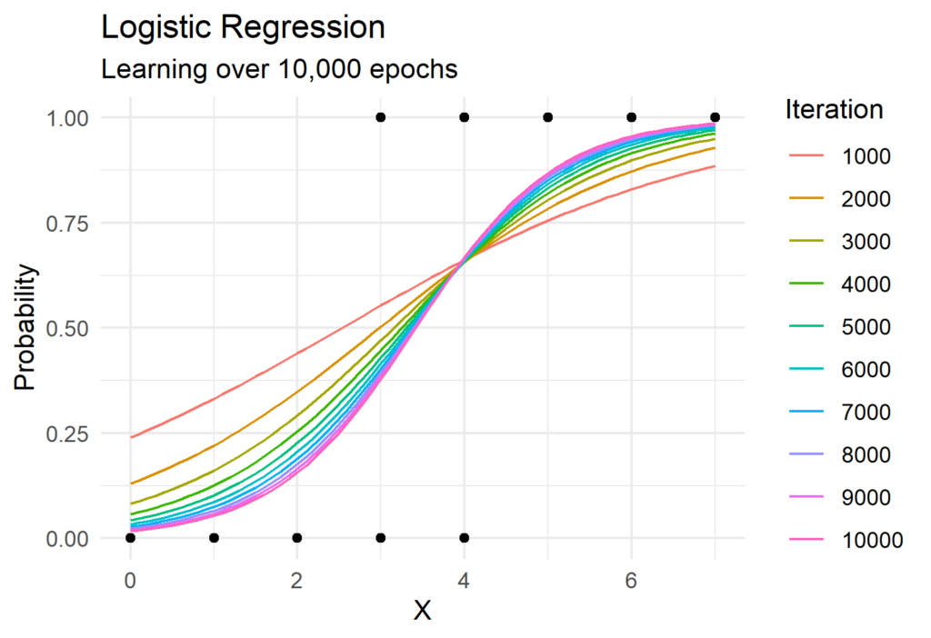
Now lets put all of this together! The Python function to perform gradient descent for logistic regression is surprisingly simple and requires the use of only Numpy. We can see gradient descent in action in the visual below which shows the predicted probabilities for each iteration.

import numpy as np

def descend(x, y, b0, b1, rate):

    # Determine x-betas
    e_xbeta = np.exp(b0 + b1 * x)
    x_probs = e_xbeta / (1 + e_xbeta)
    p_diffs = x_probs - y

    # Find gradient using partial derivative
    b0 = b0 - (rate * sum(p_diffs))
    b1 = b1 - (rate * sum(p_diffs * x))
    return b0, b1


def learn(x, y, rate=0.001, epoch=1e4):

    # Initial conditions
    b0 = 0 # Starting b0
    b1 = 0 # Starting b1
    epoch = int(epoch)

    # Arrays for coefficient history
    b0_hist = np.zeros(epoch)
    b1_hist = np.zeros(epoch)

    # Iterate over epochs
    for i in range(epoch):
        b0, b1 = descend(x, y, b0, b1, rate)
        b0_hist[i] = b0
        b1_hist[i] = b1

    # Returns history of parameters
    return b0_hist, b1_hist

# Data for train
x = np.array([0, 1, 2, 3, 4, 3, 4, 5, 6, 7])
y = np.array([0, 0, 0, 0, 0, 1, 1, 1, 1, 1])

# Generate model
b0_hist, b1_hist = learn(x, y)

Hertzsprung–Russell Diagram in D3.js

A Hertzsprung–Russell diagram (HR diagram) is a visualization of star data which shows the relationship between magnitude and spectral characteristics. The diagram was created by Ejnar Hertzsprung and Henry Norris Russell independently in the early 20th century. You can read more about these diagrams here.

While interesting, I am no astronomer and am primarily inspired by how interesting the diagrams appear. I originally saw this diagram on a post my Mike Bostock (creator of D3.js) when learning more about creating data visualizations in JavaScript. You can see his implementation here.

My visual uses the same underlying CSV as Mike Bostock’s visual, but simplifies the output and makes it smaller. It also detects user scrolls to turn individual star data points on and off to create a star-twinkle effect. The effect is most pronounced on smooth scrolls (such as a touchscreen device or trackpad).

In all, this is more of an exercise in art than data analysis. Enjoy!

Implementing KNN in Python

K-nearest neighbors (KNN) is an algorithm which identifies the k nearest data points in a training sample to a new observation. Typically, nearest is defined by the Euclidian (or straight line) distance, however, other distance norms can be used.

Python is already home to several KNN implementations the most famous of which is the scikit-learn implementation. I still believe there is value in writing your own model implementations to learn more about how they work.

First lets break down what KNN is doing visually and then code up our own implementation. The visual below (built using D3.js) shows several points which are classified into the red and blue groups.

You can hover your mouse over this visual to develop an understanding of how the nearest three points impact the classification of the point.

We can identify the three (k = 3) closest points and determine of those, which classification is the most common. The most common classification becomes our predicted value.


A few notes before we jump into our own implementation. First, it is common to use an odd number for k when performing classification to avoid ties. Second, one downside of KNN when compared to other models is that KNN must be packaged with the training data to make predictions. This is different than linear regression which only requires the coefficients to be known at the time of prediction, for example.

Now let’s look at my implementation of KNN in Python. Only 8 lines of code (excluding function imports)! A safer version of this code may also include several assertion checks to ensure inputs are of the expected type and shape.

import numpy as np
import scipy as sci

def knn(new, train, labels, k=3, mode="c"):

    distances = np.sum((new - train) ** 2, axis=1)
    k_closest = distances.argsort()[:k]
    values = np.take(labels, k_closest)
    
    if mode == "c":
        return sci.stats.mode(values)[0][0]
        
    if mode == "r":
        return np.mean(values)

Lets look at this function line by line. First, I define a function called knn which accepts a singular new observation called new, the training data called train with its associated labels (the correct prediction), and the mode which is either c for classification or r for regression.

def knn(new, train, labels, k=3, mode="c")

From there I compute how far each of the training points is from the new observation. To accurately compute the distances you would need to take the square root of this value. However, because we are only interested in the rank ordering of points, we can skip that step.

distances = np.sum((new - train) ** 2, axis=1)

Next I use argsort and take from numpy to rank order the indices by how close they are to the new observation. I use index slicing to grab the k nearest points. From there I use take to grab the values of the k closest indices from the label data.

k_closest = distances.argsort()[:k]
values = np.take(labels, k_closest)

Finally, I take the mode of the values for classification or the mean for regression. To predict over multiple observations I could pass the function into a list comprehension:

[knn(i, train, labels) for i in test]

This was a simple overview of KNN regression using basic numpy and scipy functions!

American Wealth Moves North and West

At first glance, you may think this title is referring to northwestern US states like Oregon or Idaho. While there certainly are wealthy areas in the northwestern US, I am actually referring to which parts of a given city are wealthy.

After traveling across and living in multiple parts of the United States, I have noticed that cities tend to be wealthier on their northern halves. Until now, this was just conjecture but I took the opportunity to utilize publicly available census tract data to investigate my suspicions.


Building the Visual

First, I obtained data from various public data sources. This includes census tract shapefiles, income data, and census tract to county MSA conversions.

I then selected a range of MSAs to analyze. In all I looked at Atlanta, Austin, Boston, Chicago, Dallas, Denver, Houston, Indianapolis, Kansas City, Las Vegas, Los Angeles, Miami, Milwaukee, Minneapolis, Nashville, New Orleans, New York, Oklahoma City, Orlando, Philadelphia, Phoenix, Portland, Salt Lake City, San Antonio, San Francisco, Seattle, Tampa, and Washington DC.

From there, I standardized the latitude and longitude of each MSA such that the most southwestern point in an MSA would have a coordinate of (0,0) while the most northeastern point would have a coordinate of (1,1). This controls for physical size differences between MSAs.

Lastly, I scaled the income of each census tract such that the tract with the highest income in an MSA has an income value of 1 and the lowest income tract has a value of 0. This also controls for wealth differences between MSAs.

I used this dataset to layer all of the MSA data to create a supercity that represents all of the individual MSAs collectively.

And here is the result! The closer to gold a given tract is the higher its income. Conversely, the closer to dark blue a tract is the lower its income. The black dot represents the city center. I observe a fairly clear distinction between the northwest and southeast of US cities.

There are, of course, exceptions to the rule. We can see gold census tracts in the south of some MSAs though wealth generally appears to be concentrated in the northwest.


A Simple Explanatory Model

To add some validity to these findings I estimated a very simple linear model which estimates a census tract’s income using its relative position to the city center. Here are the results:

TermCoefficient (Converted to USD)
Intercept$84,288
Longitude (West/East)-$6,963
Latitude (North/South) $7,674
Results of income prediction model

The way to read these coefficients is as follows. At the city center census tracts have, on average, a median household income of $84,288. As you move east median household income falls (hence the negative coefficient for Longitude) and as you north income rises (hence the positive coefficient for Latitude).

In other words, northwestern tracts have median household incomes approximately $14,000 wealthier than the city center or $28,000 wealthier than their southeastern counterparts.

Obviously, this model is oversimplified and would not be a good predictor of tract income given the huge variety of incomes across MSAs in the US, but it does illustrate an interesting point about income vs. tract position in an MSA.


Closing Thoughts

Before closing out, I wanted to draw attention to a few specific MSAs where this effect is particularly pronounced. I would argue that this northwest vs southeast impact is pronounced in the following six cities, especially Washington DC.

I hope this high level summary provides some interesting food for thought about the differences in income across US cities.

Kahan’s Summation Algorithm: Computing Better Sums

Suppose you have the following list of numbers in Python and you would like to compute the sum. You use the sum() function and expect it to return 0.3. Yet, when you run the code the console returns a value very slightly above 0.3:

numbers = [0.1, 0.1, 0.1]

sum(numbers)

0.30000000000000004

You can round this number of course, but it begs the question as to why the correct sum was not returned in the first place. Enter the IEEE 754 floating point standard.

Floating Point Storage

The double type is a 64 binary digit (bit) numerical storage standard that includes 1 sign bit (determines if number is positive or negative), a 53 bit significand (only 52 are stored for non-zero values), and an 11 bit exponent.

An 11 bit exponent means the smallest positive number that can be stored is 2-1022. Additionally, the largest rounding error possible in this standard is 2-52 called machine epsilon. Because this is a binary representation that means numbers that can be represented exactly in base 10 must be approximated when converting to binary.

Going back to our example above, 0.1 is a value that must be rounded for storage in this format. This is because 0.1 in binary is infinite:

0.000110011001100110011...

There are methods to store values exactly but this comes at the speed of computation. What if we want to keep the speed of 64 bit computation but reduce our error, specifically for large number series?

The Algorithm

Enter Kahan’s Summation Algorithm. Developed by William Kahan, this summation methodology allows for more accurate summation using the double storage format. Here is a simple Python implementation:

def kahan_sum(x):
   
  sum = 0.0
  c = 0.0
 
  for i in x:
    y = i - c
    t = sum + y
    c = t - sum - y
    sum = t
 
  return sum

Okay, so this looks pretty simple. But what do each of the pieces mean? The first two lines establish a function in Python while setting the starting sum and starting error to 0.0:

def kahan_sum(x):
   
  sum = 0.0
  c = 0.0

The next few lines are the for loop that iterates over each number in the list. First, any error is subtracted from the previous iteration.

y = i - c

Second, the new number is added to the running total minus any error.

t = sum + y

Third, error from this new addition is determined and the new total is assigned. This repeats until there are no more numbers.

c = t - sum - y
sum = t

A Practical Example

Okay, so the code is pretty simple but how does this work in practice? Suppose we have a list of two numbers:

[1.0, 1.0]

Step 1

The sum and error terms are set to 0.0 when the algorithm is started. The first step of each iteration is to take the current value and subtract any error from the previous iteration. Because the starting error is 0.0, we subtract 0.0 from the first value.

1.0 - 0.0 = 1.0

Step 2

Next we add the result of the previous operation to the total. Again, the initial total is 0.0 so we just add 0.0 to the value from Step 1 (1.0). Oh no! The computer had to make a rounding error. In this case, the computer was off by 0.1. We can handle this error in the next steps.

0.0 + 1.0 ~ 1.1

Step 3

In this step we determine the error from Step 2. We take the sum from Step 2 (1.1), subtract the total (0.0), and subtract the total from Step 1 (1.0). This leaves us with the approximate error.

1.1 - 0.0 - 1.0 ~ 0.1

Step 4

Finally, we record the current total for the next iteration!

1.1

And Repeat!

Now we repeat Steps 1, 2, 3, and 4 for each additional number. The difference this time is that we have non-zero values for the error and total terms. First, we subtract the error term from the last iteration to the new value:

1.0 - 0.1 = 0.9

Next, add the new value to the previous total:

1.1 + 0.9 = 2.0

Next, take the sum from the last step and subtract the previous iteration’s total and the value from the first step to estimate any error. In this case there is no error so we record a value of 0.0 for the error going into the next iteration:

2.0 - 1.1 - 0.9 = 0.0

Finally, return the sum. We can see that even though the computer made an error of 0.1, the algorithm corrected itself and returned the correct value:

2.0

Final Thoughts

Kahan’s method of summation strikes a balance between the speed of floating point arithmetic and accuracy. Hopefully this walkthrough makes the algorithm more approachable.

Association Rule Mining in R

Association rule mining is the process of determining conditional probabilities within events that contain items or characteristics. Events can range from tweets, to grocery store receipts, to credit card applications.

Items within these events should also not be unique to each event. For example, words are repeated across tweets, multiple customers will buy the same items at the grocery store, and credit card applicants will share specific characterisitcs.

For all of these applications our goal is to estimate the probability that an event will possess item B given that it has item A. This probability is also called the confidence.

In the example above we might say that we are 23% confident that a customer will purchase rice (item B) given they are purchasing chicken (item A). We can use historical transactions (events) to estimate confidence.

Now for a practical implementation using the tidyverse in R! I am using a groceries dataset from Georgia Tech. This dataset contains rows with items separated by commas.

receipt
citrus fruit, semi-finished bread
ready soups, margarine
One transaction per row with items comma separated.

Because each event contains different items I read it using readLines() and reshape into a longer format. The groceries column contains the item name while transaction contains the transaction ID.

link <- "https://cse6040.gatech.edu/datasets/groceries.csv"
groceries <- readLines(link)

# Create long form version of data
groceries_long <- 
  tibble::tibble(groceries) |>
  dplyr::mutate(
    transaction = dplyr::row_number()
  ) |>
  tidyr::separate_rows(
    groceries,
    sep = ","
  )
groceriestransaction
citrus fruit1
semi-finished bread1
tropical fruit2
Long form data with one item per row with a transaction ID.

With our data in the proper format we can develop two functions. The first function takes a vector of items and returns a vector of comma separated combinations as (A,B) and (B,A).

comb_vec <- function(items) {
  # Gets vector of all 2-level combinations
  
  p <- t(combn(items, 2))
  reg <- glue::glue("{p[, 1]},{p[, 2]}")
  rev <- glue::glue("{p[, 2]},{p[, 1]}")
  c(reg, rev)
}

For example, giving this function c("A", "B", "C") would return c("A,B" "A,C" "B,C" "B,A" "C,A" "C,B"). This is because we want to determine the probabilities of A given B and B given A.

Our final function performs the data mining. The first argument called data takes in the data frame of events and items. The last two arguments item_col and event_id tell the function which columns refer to the items and the event identifier respectively.

pair_assoc <- function(data, item_col, event_id, item_min = 1L) {
  # Derives association pairs for all elements in data
  
  # Count all items
  item_count <-
    data |>
    dplyr::count(
      A = {{ item_col }},
      name = "A Count"
    )
  
  # Get pairs as probabilities
  data |>
    dplyr::group_by({{ event_id }}) |>
    dplyr::filter(length({{ item_col }}) > 1) |>
    dplyr::reframe(comb = comb_vec({{ item_col }})) |>
    dplyr::ungroup() |>
    dplyr::count(
      comb,
      name = "A B Count"
    ) |>
    tidyr::separate(
      col = comb,
      into = c("A", "B"),
      sep = ","
    ) |>
    dplyr::left_join(
      y = item_count,
      by = "A"
    ) |>
    dplyr::mutate(
      Confidence = `A B Count` / `A Count`
    ) |>
    dplyr::arrange(desc(Confidence))
}

This function works in two stages. First, it determines the count of all individual items in the data set. In the example with groceries, this might be the counts of transactions with rice, beans, etc.

groceriesA Count
baking powder174
berries327
Counts of individual items serve as the denominator in the confidence computation.

The second stage uses the comb_vec() function to determine all valid item combinations within each group. This stage only returns valid combinations where the confidence is > 0%.

Finally, the function left joins the item counts to the combination counts and computes the confidence values. I called the function and return the result. I am also filtering to only combinations with a confidence of 50% or more with items purchased more than 10 times.

groceries_long |>
  pair_assoc(
    item_col = groceries, 
    event_id = transaction
  ) |>
  dplyr::filter(
    `A Count` >= 10,
    Confidence >= 0.5
  )

Here we can see the head of the results table ordered by confidence from highest to lowest. We observe that the confidence of honey and whole milk is 73%! In other words, 73% of the transactions that contain honey also contain whole milk.

ABA B CountA CountConfidence
honeywhole milk11140.733
frozen fruitsother vegetables8120.667
cerealswhole milk36560.643
ricewhole milk46750.613
Head of results table.

Association rule mining is a fairly simple and easy to interpret technique to help draw relationships between items and events in a data set.