Gradient Descent for Logistic Regression

Unlike linear regression, logistic regression does not have a closed-form solution. Instead, we use the generalized linear model approach using gradient descent and maximum likelihood.

First, lets discuss logistic regression. Unlike linear regression, values in logistic regression generally take two forms, log-odds and probability. Log-odds is the value returned when we multiply each term by its coefficient and sum the results. This value can span from -Inf to Inf.

Probability form takes the log-odds form and squishes it to values between 0 and 1. This is important because logistic regression is a binary classification method which returns the probability of an event occurring.

To transform log-odds to a probability we perform the following operation: exp(log-odds) / 1 + exp(log-odds). And to transform probability back to log odds we perform the following operation: log(probability / 1 – probability).


Next, we need to consider our cost function. All generalized linear models have a cost function. For logistic regression, we maximize likelihood. To compute the likelihood of a set of coefficients we perform the following operations: sum(log(probability)) for data points with a true classification of 1 and sum(log(1 – probability)) for data points with a true classification of 0.

Even though we can compute the given cost of a set of parameters, how can we determine which direction will improve our outcome? It turns out we can take the partial derivative for each parameter (b0, b1, … bn) and nudge our parameters into the right direction.


Suppose we have a simple logistic regression model with only two parameters, b0 (the intercept) and b1 (the relationship between x and y). We would compute the gradient of our parameters using the following operations: b0 – rate * sum(probability – class) for the intercept and b1 – rate * sum((probability – class) * x)) for the relationship between x and y.

Note that rate above is the learning rate. A larger learning rate will nudge the coefficients more quickly where a smaller learning rate will approach the coefficients more slowly, but may achieve better estimates.


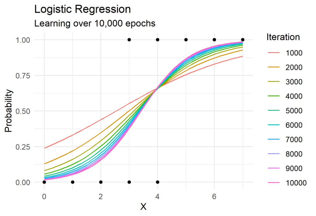
Now lets put all of this together! The Python function to perform gradient descent for logistic regression is surprisingly simple and requires the use of only Numpy. We can see gradient descent in action in the visual below which shows the predicted probabilities for each iteration.

import numpy as np

def descend(x, y, b0, b1, rate):

    # Determine x-betas
    e_xbeta = np.exp(b0 + b1 * x)
    x_probs = e_xbeta / (1 + e_xbeta)
    p_diffs = x_probs - y

    # Find gradient using partial derivative
    b0 = b0 - (rate * sum(p_diffs))
    b1 = b1 - (rate * sum(p_diffs * x))
    return b0, b1


def learn(x, y, rate=0.001, epoch=1e4):

    # Initial conditions
    b0 = 0 # Starting b0
    b1 = 0 # Starting b1
    epoch = int(epoch)

    # Arrays for coefficient history
    b0_hist = np.zeros(epoch)
    b1_hist = np.zeros(epoch)

    # Iterate over epochs
    for i in range(epoch):
        b0, b1 = descend(x, y, b0, b1, rate)
        b0_hist[i] = b0
        b1_hist[i] = b1

    # Returns history of parameters
    return b0_hist, b1_hist

# Data for train
x = np.array([0, 1, 2, 3, 4, 3, 4, 5, 6, 7])
y = np.array([0, 0, 0, 0, 0, 1, 1, 1, 1, 1])

# Generate model
b0_hist, b1_hist = learn(x, y)

Hertzsprung–Russell Diagram in D3.js

A Hertzsprung–Russell diagram (HR diagram) is a visualization of star data which shows the relationship between magnitude and spectral characteristics. The diagram was created by Ejnar Hertzsprung and Henry Norris Russell independently in the early 20th century. You can read more about these diagrams here.

While interesting, I am no astronomer and am primarily inspired by how interesting the diagrams appear. I originally saw this diagram on a post my Mike Bostock (creator of D3.js) when learning more about creating data visualizations in JavaScript. You can see his implementation here.

My visual uses the same underlying CSV as Mike Bostock’s visual, but simplifies the output and makes it smaller. It also detects user scrolls to turn individual star data points on and off to create a star-twinkle effect. The effect is most pronounced on smooth scrolls (such as a touchscreen device or trackpad).

In all, this is more of an exercise in art than data analysis. Enjoy!

American Wealth Moves North and West

At first glance, you may think this title is referring to northwestern US states like Oregon or Idaho. While there certainly are wealthy areas in the northwestern US, I am actually referring to which parts of a given city are wealthy.

After traveling across and living in multiple parts of the United States, I have noticed that cities tend to be wealthier on their northern halves. Until now, this was just conjecture but I took the opportunity to utilize publicly available census tract data to investigate my suspicions.


Building the Visual

First, I obtained data from various public data sources. This includes census tract shapefiles, income data, and census tract to county MSA conversions.

I then selected a range of MSAs to analyze. In all I looked at Atlanta, Austin, Boston, Chicago, Dallas, Denver, Houston, Indianapolis, Kansas City, Las Vegas, Los Angeles, Miami, Milwaukee, Minneapolis, Nashville, New Orleans, New York, Oklahoma City, Orlando, Philadelphia, Phoenix, Portland, Salt Lake City, San Antonio, San Francisco, Seattle, Tampa, and Washington DC.

From there, I standardized the latitude and longitude of each MSA such that the most southwestern point in an MSA would have a coordinate of (0,0) while the most northeastern point would have a coordinate of (1,1). This controls for physical size differences between MSAs.

Lastly, I scaled the income of each census tract such that the tract with the highest income in an MSA has an income value of 1 and the lowest income tract has a value of 0. This also controls for wealth differences between MSAs.

I used this dataset to layer all of the MSA data to create a supercity that represents all of the individual MSAs collectively.

And here is the result! The closer to gold a given tract is the higher its income. Conversely, the closer to dark blue a tract is the lower its income. The black dot represents the city center. I observe a fairly clear distinction between the northwest and southeast of US cities.

There are, of course, exceptions to the rule. We can see gold census tracts in the south of some MSAs though wealth generally appears to be concentrated in the northwest.


A Simple Explanatory Model

To add some validity to these findings I estimated a very simple linear model which estimates a census tract’s income using its relative position to the city center. Here are the results:

TermCoefficient (Converted to USD)
Intercept$84,288
Longitude (West/East)-$6,963
Latitude (North/South) $7,674
Results of income prediction model

The way to read these coefficients is as follows. At the city center census tracts have, on average, a median household income of $84,288. As you move east median household income falls (hence the negative coefficient for Longitude) and as you north income rises (hence the positive coefficient for Latitude).

In other words, northwestern tracts have median household incomes approximately $14,000 wealthier than the city center or $28,000 wealthier than their southeastern counterparts.

Obviously, this model is oversimplified and would not be a good predictor of tract income given the huge variety of incomes across MSAs in the US, but it does illustrate an interesting point about income vs. tract position in an MSA.


Closing Thoughts

Before closing out, I wanted to draw attention to a few specific MSAs where this effect is particularly pronounced. I would argue that this northwest vs southeast impact is pronounced in the following six cities, especially Washington DC.

I hope this high level summary provides some interesting food for thought about the differences in income across US cities.

Kahan’s Summation Algorithm: Computing Better Sums

Suppose you have the following list of numbers in Python and you would like to compute the sum. You use the sum() function and expect it to return 0.3. Yet, when you run the code the console returns a value very slightly above 0.3:

numbers = [0.1, 0.1, 0.1]

sum(numbers)

0.30000000000000004

You can round this number of course, but it begs the question as to why the correct sum was not returned in the first place. Enter the IEEE 754 floating point standard.

Floating Point Storage

The double type is a 64 binary digit (bit) numerical storage standard that includes 1 sign bit (determines if number is positive or negative), a 53 bit significand (only 52 are stored for non-zero values), and an 11 bit exponent.

An 11 bit exponent means the smallest positive number that can be stored is 2-1022. Additionally, the largest rounding error possible in this standard is 2-52 called machine epsilon. Because this is a binary representation that means numbers that can be represented exactly in base 10 must be approximated when converting to binary.

Going back to our example above, 0.1 is a value that must be rounded for storage in this format. This is because 0.1 in binary is infinite:

0.000110011001100110011...

There are methods to store values exactly but this comes at the speed of computation. What if we want to keep the speed of 64 bit computation but reduce our error, specifically for large number series?

The Algorithm

Enter Kahan’s Summation Algorithm. Developed by William Kahan, this summation methodology allows for more accurate summation using the double storage format. Here is a simple Python implementation:

def kahan_sum(x):
   
  sum = 0.0
  c = 0.0
 
  for i in x:
    y = i - c
    t = sum + y
    c = t - sum - y
    sum = t
 
  return sum

Okay, so this looks pretty simple. But what do each of the pieces mean? The first two lines establish a function in Python while setting the starting sum and starting error to 0.0:

def kahan_sum(x):
   
  sum = 0.0
  c = 0.0

The next few lines are the for loop that iterates over each number in the list. First, any error is subtracted from the previous iteration.

y = i - c

Second, the new number is added to the running total minus any error.

t = sum + y

Third, error from this new addition is determined and the new total is assigned. This repeats until there are no more numbers.

c = t - sum - y
sum = t

A Practical Example

Okay, so the code is pretty simple but how does this work in practice? Suppose we have a list of two numbers:

[1.0, 1.0]

Step 1

The sum and error terms are set to 0.0 when the algorithm is started. The first step of each iteration is to take the current value and subtract any error from the previous iteration. Because the starting error is 0.0, we subtract 0.0 from the first value.

1.0 - 0.0 = 1.0

Step 2

Next we add the result of the previous operation to the total. Again, the initial total is 0.0 so we just add 0.0 to the value from Step 1 (1.0). Oh no! The computer had to make a rounding error. In this case, the computer was off by 0.1. We can handle this error in the next steps.

0.0 + 1.0 ~ 1.1

Step 3

In this step we determine the error from Step 2. We take the sum from Step 2 (1.1), subtract the total (0.0), and subtract the total from Step 1 (1.0). This leaves us with the approximate error.

1.1 - 0.0 - 1.0 ~ 0.1

Step 4

Finally, we record the current total for the next iteration!

1.1

And Repeat!

Now we repeat Steps 1, 2, 3, and 4 for each additional number. The difference this time is that we have non-zero values for the error and total terms. First, we subtract the error term from the last iteration to the new value:

1.0 - 0.1 = 0.9

Next, add the new value to the previous total:

1.1 + 0.9 = 2.0

Next, take the sum from the last step and subtract the previous iteration’s total and the value from the first step to estimate any error. In this case there is no error so we record a value of 0.0 for the error going into the next iteration:

2.0 - 1.1 - 0.9 = 0.0

Finally, return the sum. We can see that even though the computer made an error of 0.1, the algorithm corrected itself and returned the correct value:

2.0

Final Thoughts

Kahan’s method of summation strikes a balance between the speed of floating point arithmetic and accuracy. Hopefully this walkthrough makes the algorithm more approachable.

Association Rule Mining in R

Association rule mining is the process of determining conditional probabilities within events that contain items or characteristics. Events can range from tweets, to grocery store receipts, to credit card applications.

Items within these events should also not be unique to each event. For example, words are repeated across tweets, multiple customers will buy the same items at the grocery store, and credit card applicants will share specific characterisitcs.

For all of these applications our goal is to estimate the probability that an event will possess item B given that it has item A. This probability is also called the confidence.

In the example above we might say that we are 23% confident that a customer will purchase rice (item B) given they are purchasing chicken (item A). We can use historical transactions (events) to estimate confidence.

Now for a practical implementation using the tidyverse in R! I am using a groceries dataset from Georgia Tech. This dataset contains rows with items separated by commas.

receipt
citrus fruit, semi-finished bread
ready soups, margarine
One transaction per row with items comma separated.

Because each event contains different items I read it using readLines() and reshape into a longer format. The groceries column contains the item name while transaction contains the transaction ID.

link <- "https://cse6040.gatech.edu/datasets/groceries.csv"
groceries <- readLines(link)

# Create long form version of data
groceries_long <- 
  tibble::tibble(groceries) |>
  dplyr::mutate(
    transaction = dplyr::row_number()
  ) |>
  tidyr::separate_rows(
    groceries,
    sep = ","
  )
groceriestransaction
citrus fruit1
semi-finished bread1
tropical fruit2
Long form data with one item per row with a transaction ID.

With our data in the proper format we can develop two functions. The first function takes a vector of items and returns a vector of comma separated combinations as (A,B) and (B,A).

comb_vec <- function(items) {
  # Gets vector of all 2-level combinations
  
  p <- t(combn(items, 2))
  reg <- glue::glue("{p[, 1]},{p[, 2]}")
  rev <- glue::glue("{p[, 2]},{p[, 1]}")
  c(reg, rev)
}

For example, giving this function c("A", "B", "C") would return c("A,B" "A,C" "B,C" "B,A" "C,A" "C,B"). This is because we want to determine the probabilities of A given B and B given A.

Our final function performs the data mining. The first argument called data takes in the data frame of events and items. The last two arguments item_col and event_id tell the function which columns refer to the items and the event identifier respectively.

pair_assoc <- function(data, item_col, event_id, item_min = 1L) {
  # Derives association pairs for all elements in data
  
  # Count all items
  item_count <-
    data |>
    dplyr::count(
      A = {{ item_col }},
      name = "A Count"
    )
  
  # Get pairs as probabilities
  data |>
    dplyr::group_by({{ event_id }}) |>
    dplyr::filter(length({{ item_col }}) > 1) |>
    dplyr::reframe(comb = comb_vec({{ item_col }})) |>
    dplyr::ungroup() |>
    dplyr::count(
      comb,
      name = "A B Count"
    ) |>
    tidyr::separate(
      col = comb,
      into = c("A", "B"),
      sep = ","
    ) |>
    dplyr::left_join(
      y = item_count,
      by = "A"
    ) |>
    dplyr::mutate(
      Confidence = `A B Count` / `A Count`
    ) |>
    dplyr::arrange(desc(Confidence))
}

This function works in two stages. First, it determines the count of all individual items in the data set. In the example with groceries, this might be the counts of transactions with rice, beans, etc.

groceriesA Count
baking powder174
berries327
Counts of individual items serve as the denominator in the confidence computation.

The second stage uses the comb_vec() function to determine all valid item combinations within each group. This stage only returns valid combinations where the confidence is > 0%.

Finally, the function left joins the item counts to the combination counts and computes the confidence values. I called the function and return the result. I am also filtering to only combinations with a confidence of 50% or more with items purchased more than 10 times.

groceries_long |>
  pair_assoc(
    item_col = groceries, 
    event_id = transaction
  ) |>
  dplyr::filter(
    `A Count` >= 10,
    Confidence >= 0.5
  )

Here we can see the head of the results table ordered by confidence from highest to lowest. We observe that the confidence of honey and whole milk is 73%! In other words, 73% of the transactions that contain honey also contain whole milk.

ABA B CountA CountConfidence
honeywhole milk11140.733
frozen fruitsother vegetables8120.667
cerealswhole milk36560.643
ricewhole milk46750.613
Head of results table.

Association rule mining is a fairly simple and easy to interpret technique to help draw relationships between items and events in a data set.