Unlike linear regression, logistic regression does not have a closed-form solution. Instead, we use the generalized linear model approach using gradient descent and maximum likelihood.
First, lets discuss logistic regression. Unlike linear regression, values in logistic regression generally take two forms, log-odds and probability. Log-odds is the value returned when we multiply each term by its coefficient and sum the results. This value can span from -Inf to Inf.
Probability form takes the log-odds form and squishes it to values between 0 and 1. This is important because logistic regression is a binary classification method which returns the probability of an event occurring.
To transform log-odds to a probability we perform the following operation: exp(log-odds) / 1 + exp(log-odds). And to transform probability back to log odds we perform the following operation: log(probability / 1 – probability).
Next, we need to consider our cost function. All generalized linear models have a cost function. For logistic regression, we maximize likelihood. To compute the likelihood of a set of coefficients we perform the following operations: sum(log(probability)) for data points with a true classification of 1 and sum(log(1 – probability)) for data points with a true classification of 0.
Even though we can compute the given cost of a set of parameters, how can we determine which direction will improve our outcome? It turns out we can take the partial derivative for each parameter (b0, b1, … bn) and nudge our parameters into the right direction.
Suppose we have a simple logistic regression model with only two parameters, b0 (the intercept) and b1 (the relationship between x and y). We would compute the gradient of our parameters using the following operations: b0 – rate * sum(probability – class) for the intercept and b1 – rate * sum((probability – class) * x)) for the relationship between x and y.
Note that rate above is the learning rate. A larger learning rate will nudge the coefficients more quickly where a smaller learning rate will approach the coefficients more slowly, but may achieve better estimates.
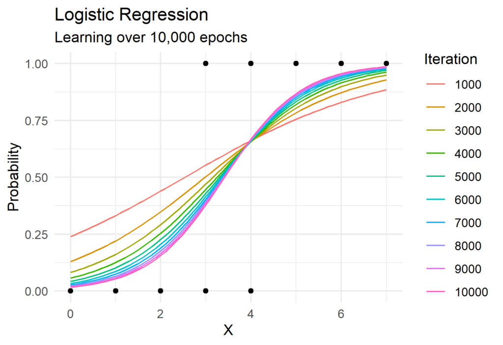
Now lets put all of this together! The Python function to perform gradient descent for logistic regression is surprisingly simple and requires the use of only Numpy. We can see gradient descent in action in the visual below which shows the predicted probabilities for each iteration.
import numpy as np

def descend(x, y, b0, b1, rate):

    # Determine x-betas
    e_xbeta = np.exp(b0 + b1 * x)
    x_probs = e_xbeta / (1 + e_xbeta)
    p_diffs = x_probs - y

    # Find gradient using partial derivative
    b0 = b0 - (rate * sum(p_diffs))
    b1 = b1 - (rate * sum(p_diffs * x))
    return b0, b1


def learn(x, y, rate=0.001, epoch=1e4):

    # Initial conditions
    b0 = 0 # Starting b0
    b1 = 0 # Starting b1
    epoch = int(epoch)

    # Arrays for coefficient history
    b0_hist = np.zeros(epoch)
    b1_hist = np.zeros(epoch)

    # Iterate over epochs
    for i in range(epoch):
        b0, b1 = descend(x, y, b0, b1, rate)
        b0_hist[i] = b0
        b1_hist[i] = b1

    # Returns history of parameters
    return b0_hist, b1_hist

# Data for train
x = np.array([0, 1, 2, 3, 4, 3, 4, 5, 6, 7])
y = np.array([0, 0, 0, 0, 0, 1, 1, 1, 1, 1])

# Generate model
b0_hist, b1_hist = learn(x, y)
